Home Energy Consumption
This first tutorial explains how to use Maki Nage for basic feature engineering on time-series data, and how to deploy a model operating in streaming mode. The task of this tutorial is a regression: We will predict the power consumption of a house, based on weather information.
Important
Maki Nage is designed to work efficiently with pypy. Please ensure that you use it as your interpreter for better performance.
The dataset
In this example, we will work on the Smart Home Dataset. It can be downloaded from kaggle here.
The dataset is a CSV file of 130MB, its content looks like this:
$ head HomeC.csv
time,use [kW],gen [kW],House overall [kW],Dishwasher [kW],Furnace 1 [kW],Furnace 2 [kW],Home office [kW],Fridge [kW],Wine cellar [kW],Garage door [kW],Kitchen 12 [kW],Kitchen 14 [kW],Kitchen 38 [kW],Barn [kW],Well [kW],Microwave [kW],Living room [kW],Solar [kW],temperature,icon,humidity,visibility,summary,apparentTemperature,pressure,windSpeed,cloudCover,windBearing,precipIntensity,dewPoint,precipProbability
1451624400,0.932833333,0.003483333,0.932833333,3.33E-05,0.0207,0.061916667,0.442633333,0.12415,0.006983333,0.013083333,0.000416667,0.00015,0,0.03135,0.001016667,0.004066667,0.001516667,0.003483333,36.14,clear-night,0.62,10,Clear,29.26,1016.91,9.18,cloudCover,282,0,24.4,0
1451624401,0.934333333,0.003466667,0.934333333,0,0.020716667,0.063816667,0.444066667,0.124,0.006983333,0.013116667,0.000416667,0.00015,0,0.0315,0.001016667,0.004066667,0.00165,0.003466667,36.14,clear-night,0.62,10,Clear,29.26,1016.91,9.18,cloudCover,282,0,24.4,0
1451624402,0.931816667,0.003466667,0.931816667,1.67E-05,0.0207,0.062316667,0.446066667,0.123533333,0.006983333,0.013083333,0.000433333,0.000166667,1.67E-05,0.031516667,0.001,0.004066667,0.00165,0.003466667,36.14,clear-night,0.62,10,Clear,29.26,1016.91,9.18,cloudCover,282,0,24.4,0
For simplicity, We will use only a few columns:
House overall: This is the label we want to predict, the total energy consumption of the house.
temperature: The weather temperature in °F.
pressure: The atmospheric pressure in hPa (hectopascal).
windSpeed: The wind speed.
We will use the following imports:
from collections import namedtuple
import rx
import rx.operators as ops
import rxsci as rs
import rxsci.container.csv as csv
import distogram
The recommended data type when working with Maki Nage is namedtuple, hence the first import. Then there are two RxPy imports. Since Maki Nage is based on ReactiveX, we will use some ReactiveX operators. Then is the main RxSci import, and another one to work with CSV files. RxSci is the Maki Nage library that implements all transformation functions. It is the library that you will mostly use in a Maki Nage application. The final import is used for the data exploration phase when computing statistics on the data distributions.
With these imports, we can start a template code that will read the CSV file. The first step consists of defining the schema of this CSV file:
dataset_path = '/opt/dataset/HomeC.csv'
parser = csv.create_line_parser(
    dtype=[
        ('time', 'int'),
        ('use', 'float'),
        ('gen', 'float'),
        ('house_overall', 'float'),
        ('dishwasher', 'float'),
        ('furnace1', 'float'),
        ('furnace2', 'float'),
        ('home_office', 'float'),
        ('fridge', 'float'),
        ('wine_cellar', 'float'),
        ('garage_door', 'float'),
        ('kitchen_12', 'float'),
        ('kitchen_14', 'float'),
        ('kitchen_38', 'float'),
        ('barn', 'float'),
        ('well', 'float'),
        ('microwave', 'float'),
        ('living_room', 'float'),
        ('solar', 'float'),
        ('temperature', 'float'),
        ('icon', 'str'),
        ('humidity', 'float'),
        ('visibility', 'float'),
        ('summary', 'str'),
        ('apparent_temperature', 'float'),
        ('pressure', 'float'),
        ('wind_speed', 'float'),
        ('cloud_cover', 'str'),
        ('wind_bearing', 'float'),
        ('precip_intensity', 'float'),
        ('dew_point', 'float'),
        ('precip_probability', 'float'),
    ]
)
Then, loading and processing its content is done the following way:
csv.load_from_file(dataset_path, parser).pipe().run()
Many things happen on this single line: The load_from_file function is a factory operator that creates an Observable from the content of the CSV file. An Observable is the term used for a stream of events. The Observable will emit one item - one event - for each line of the CSV file. The load_from_file operator takes two arguments: the path of the CSV file and its schema.
The pipe operator one of the two operators that you will use most frequently: It allows you to create chains of operators, so that data transformations can be done sequentially. For now, no sequence is provided, so no transformation is done.
Finally, the run operator subscribes to the Observable. Calling it triggers the actual execution of the whole computation graph.
Now that we have our CSV dataset available as an Observable, let’s work on it!
Data Exploration
Overall Consumption
As a first step, let’s compute some statistics on the house overall column, and plot its histogram. For these two steps, we need to compute a compressed representation of the data distribution. This is done by creating a graph that consists of two operators:
dist = csv.load_from_file(dataset_path, parser).pipe(
    rs.ops.map(lambda i: i.house_overall),
    rs.math.dist.update(reduce=True),
).run()
The map operator applies a transformation function for each item emitted by the source Observable. Note that all operators take observables as input and return Observables as output. This allows to chain operators very easily.
The second operator is math.dist.update. It computes a compressed representation of the data distribution that can be used to compute statistics on it, such as mean, variance, and quantiles. The reduce parameter indicates that we want the operator to emit an item only when the source Observable completes, i.e. when all items have been processed. The default behavior is to emit a distribution object for each item received as input.
As said previously, the run operator subscribes to the resulting Observable. Moreover, it returns that last item emitted. On our graph, this is the distribution object.
From this object, we can do several statistical analyses. Computing classical statistical information is done with the describe operator:
print("house overall consumption statistics:")
print(rx.just(dist).pipe(
    rs.math.dist.describe(),
).run())
Note that we still have the same structure here, always working with Observables: First an observable is created from the dist object, with the just operator. This observable will emit a single item. This may seem unnecessarily complex at first, but when working in a streaming way, this is just a particular case of a stream. The important point is that all the operators that we use work on Observables, whether they emit no item, some items, or an infinite number of items.
The math.dist.describe operator emits a namedtuple with the following statistics for each item it receives:
min |
0.0 |
max |
14.71456667 |
mean |
0.8589623950050789 |
stddev |
1.0574552803110226 |
p25 |
0.36709267099355347 |
p50 |
0.568152839202991 |
p75 |
0.9730122941873172 |
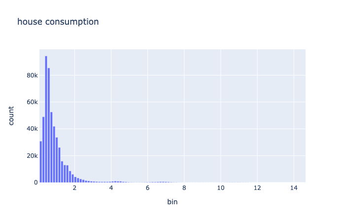
Another kind of information that can be computed from the dist object is the histogram of the distribution. For this, we use once again the same pattern:
df_hist = rx.just(dist).pipe(
    rs.math.dist.histogram(),
    rs.ops.map(lambda i: pd.DataFrame(np.array(i), columns=["bin", "count"])),
).run()

fig = px.bar(df_hist, x="bin", y="count", title="house consumption")
fig.update_layout(height=300)
fig.show()
The math.dist.histogram operator computes the histogram of the distribution. Then this histogram object is mapped to a pandas dataframe so that it can be used by plotly. The resulting plot is:
Multiple Variables Exploration
In the previous section, we studied one feature. The first step consisted of computing a compressed representation of the data distribution by using two operators:
rs.ops.map(lambda i: i.house_overall),
rs.math.dist.update(reduce=True),
Now we want to do the same for other columns. One naive way is to do the same steps for each feature. However, this means that we need to process the dataset as many times as the features we have. Fortunately, all these steps can be done in parallel, thanks to a dedicated operator: tee_map. The tee_map operator applies several transformation graphs to the same source of data in parallel. So if we want to compute four distributions on a single reading pass, we can do the following:
dist = csv.load_from_file(dataset_path, parser).pipe(
    rs.ops.tee_map(
        rx.pipe(  # graph 1
            rs.ops.map(lambda i: i.house_overall),
            rs.math.dist.update(reduce=True),
        ),
        rx.pipe(  # graph 2
            rs.ops.map(lambda i: i.temperature),
            rs.math.dist.update(reduce=True),
        ),
        rx.pipe(  # graph 3
            rs.ops.map(lambda i: i.pressure),
            rs.math.dist.update(reduce=True),
        ),
        rx.pipe(  # graph 4
            rs.ops.map(lambda i: i.wind_speed),
            rs.math.dist.update(reduce=True),
        ),
    )
).run()
Here we have four computation graphs - one for each feature - that are processed in parallel. The final dist variable is a tuple of four fields, one for each computation graph:
print(dist)
(<distogram.Distogram object at 0x000000000af063d8>,
<distogram.Distogram object at 0x0000000008ca7b78>,
<distogram.Distogram object at 0x0000000008ca7478>,
<distogram.Distogram object at 0x0000000008ca6f00>)
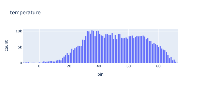
From these dist objects, we can now print the statistics and histogram of the columns are previously:
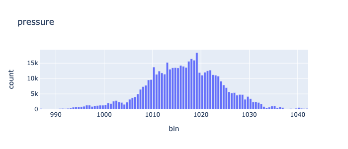
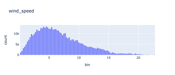
cols = ['house_overall', 'temperature', 'pressure', 'wind_speed']


for i in range(4):
    print("{} statistics:".format(cols[i]))
    print(rx.just(dist[i]).pipe(
        rs.math.dist.describe(),
    ).run())

    df_hist = rx.just(dist[i]).pipe(
        rs.math.dist.histogram(),
        rs.ops.map(lambda i: pd.DataFrame(np.array(i), columns=["bin", "count"])),
    ).run()

    fig = px.bar(df_hist, x="bin", y="count", title=cols[i])
    fig.update_layout(height=300)
    fig.show()
min |
0.0 |
max |
14.71456667 |
mean |
0.8589623950050789 |
stddev |
1.0574552803110226 |
p25 |
0.36709267099355347 |
p50 |
0.568152839202991 |
p75 |
0.9730122941873172 |
min |
-11.45 |
max |
93.72 |
mean |
50.74525179099427 |
stddev |
19.10129528623627 |
p25 |
35.774367229171965 |
p50 |
50.37779947700175 |
p75 |
66.26310350773754 |
min |
986.4 |
max |
1042.46 |
mean |
1016.3016253696112 |
stddev |
7.893601267311901 |
p25 |
1011.2888478205701 |
p50 |
1016.5285369580786 |
p75 |
1021.4751151837601 |
min |
0.0 |
max |
22.91 |
mean |
6.649935544045547 |
stddev |
3.9822204733738173 |
p25 |
3.665238739924194 |
p50 |
5.923371960965267 |
p75 |
8.936888719278361 |
Feature Engineering
Now let’s work on the features. We will use three feature for the model:
The ratio between pressure and wind speed.
The temperature value
The standard deviation of the temperature on the previous 6 hours.
Moreover, we will compute one feature for each hour. Since the dataset has been sampled every minute, we will reduce the size of a ratio of 60. Let’s work on this step by step. The first thing is to declare a data type for these features:
Features = namedtuple('Features', ['label', 'pspeed_ratio', 'temperature', 'temperature_stddev'])
As a first step, we can compute the pressure/speed ratio, and save the current temperature:
epsilon = 1e-5
features = csv.load_from_file(dataset_path, parser).pipe(
    rs.ops.map(lambda i: Features(
        label=i.house_overall,
        pspeed_ratio=i.pressure / (i.wind_speed + epsilon),
        temperature=i.temperature,
        temperature_stddev=0.0,
    )),
).run()
The input of the map operator is items for each line of the dataset, the output is Feature items, one for each entry in the dataset. Note that the temperature standard deviation is set to 0 for now.
The second step is to compute a rolling window of 6 hours, with a stride of one hour. This is a type of transformation that is hard - or impossible - to implement in most dataframe oriented frameworks. RxSci has a dedicated operator for this common operation on time series: roll. It takes three arguments as input: The size of the window, the size of stride, and the computation graph.
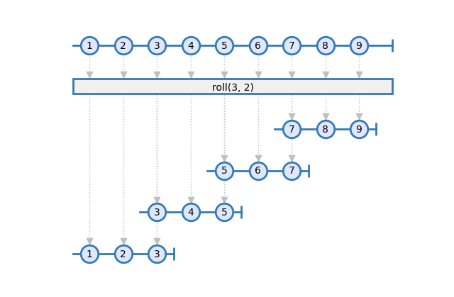
Here is how we can use it:
rs.data.roll(window=60*6, stride=60, a_pipeline)
We need a pipeline that returns the last value of pspeed_ratio and temperature on one side, and the standard deviation of the temperature on the other side. So we also need the tee_map operator to compute them in parallel:
rs.ops.tee_map(
    rs.ops.last(),
    rs.math.stddev(lambda i: i.temperature, reduce=True),
)
This computation graph returns the last item emitted by the source observable and the standard deviation of the temperature field. We can now use it in the rolling window:
rs.data.roll(
    window=60*6, stride=60,
    pipeline=rs.ops.tee_map(
        rs.ops.last(),
        rs.math.stddev(lambda i: i.temperature, reduce=True),
    )
),
The roll operator creates a new Observable for each window, so the tee_map computation is done for each of these generated windows.
The complete code is:
Features = namedtuple('Features', ['label', 'pspeed_ratio', 'temperature', 'temperature_stddev'])
epsilon = 1e-5
df = csv.load_from_file(dataset_path, parser).pipe(
    rs.ops.map(lambda i: Features(
        label=i.house_overall,
        pspeed_ratio=i.pressure / (i.wind_speed + epsilon),
        temperature=i.temperature,
        temperature_stddev=0.0,
    )),
    rs.state.with_memory_store(rx.pipe(
        rs.data.roll(
            window=60*6, stride=60,
            pipeline=rs.ops.tee_map(
                rs.ops.last(),
                rs.math.stddev(lambda i: i.temperature, reduce=True),
            )
        ),
    )),
    rs.ops.map(lambda i: Features(i[0].label, i[0].pspeed_ratio, i[0].temperature, i[1])),
    rs.ops.to_pandas()
).run()
todo: reactivity diagram
There are several other additions to this code. First, the roll operator can be used only within the context of a state store. The reason is that roll is one of the operators that work only on MuxObservables, a specialized implementation of Observables optimized for aggregate and stateful transforms.
Then the final map transformation may require some clarifications. Its source Observable contains tuples emitted by the roll operator. These are tuples of two fields. The first one is the last Features item received on each window. The second one is the temperature standard deviation. So the map operator creates new feature items from the label, pspeed_ratio, and temperature from the first element; and the standard deviation from the second element.
Finally, the to_pandas operator transforms the final Observable into a pandas dataframe. This is a way to get out of RxSci and continue the processing with other tools.
Training
This step does not involve Maki Nage but we present it as an end-to-end example. We will use a linear regression from scikit-learn:
model = Ridge(alpha=0.5)

x = df[['pspeed_ratio', 'temperature', 'temperature_stddev']]
y = df['label']
x_train, x_test, y_train, y_test = train_test_split(x, y, test_size=0.2)

model.fit(x_train, y_train)
And print the RMSE of the generated model:
pred = model.predict(x_test)
print(np.sqrt(mean_squared_error(y_test,pred)))
0.9800074715106518
Deployment
Maki Nage comes with tools to ease the deployment of data transformation and models. This part is based on Kafka, a distributed streaming platform. Kafka requires a broker to be installed, usually on a cluster. For tests or work on a single machine, you can use the docker environment provided by Maki Nage. Let’s start a local Kafka cluster:
git clone https://github.com/maki-nage/docker.git
cd docker/compose/mn-dev
docker-compose up -d kafka
Deployment requires that the code is available as a python package. You can retrieve and install a package containing the code of all examples this way:
git clone https://github.com/maki-nage/makinage-examples.git
cd makinage-examples
python setup.py develop
Feature Engineering
The feature engineering code for the deployment is the following:
def compute_house_features(config, data):
    epsilon = 1e-5
    features = data.pipe(
        csv.load(parser),
        rs.ops.map(lambda i: Features(
            label=i.house_overall,
            pspeed_ratio=i.pressure / (i.wind_speed + epsilon),
            temperature=i.temperature,
            temperature_stddev=0.0,
        )),
        rs.state.with_memory_store(rx.pipe(
            rs.data.roll(
                window=60*6, stride=60,
                pipeline=rs.ops.tee_map(
                    rs.ops.last(),
                    rs.math.stddev(lambda i: i.temperature, reduce=True),
                )
            ),
        )),
        rs.ops.map(lambda i: Features(i[0].label, i[0].pspeed_ratio, i[0].temperature, i[1])),
    )

    return features,
This is the same code that we wrote during the feature engineering part, with only 4 minor changes.
First, the code is embedded in a function taking two arguments: The first one is an Observable of the configuration of the application (its usage is explained later). The second one is an Observable of the data. Each row is received from this observable instead of being read from a file.
As a consequence, the second change is that the CSV is not read from the file, but each row is parsed from the data Observable. The csv.load operator is used instead of csv.load_from_file.
The third change is the removal of the to_list operator: There is no need to aggregate all items in a single list. The application work in streaming mode: The is a stream of events as input (the rows of the CSV dataset), and it returns a stream of events (the computed features). The source and the sink are Kafka topics. If you are not familiar with Kafka, you can consider for now that a Kafka topic is equivalent to an Observable.
The last change is the fact that we return a tuple, containing the output Observables of the application. In this case, there is a single Observable.
To execute this application, a configuration file is needed. This YAML file contains information on how to execute the application:
application:
    name: house_features
kafka:
    endpoint: "localhost"
topics:
    - name: house_values
        encoder: makinage.encoding.string
        start_from: beginning
    - name: house_features
        encoder: makinage.encoding.json
operators:
    compute_house_features:
        factory: makinage_examples.house.features:compute_house_features
        sources:
            - house_values
        sinks:
            - house_features
The application section defines the name of the application. The kafka section contains the Kafka cluster configuration. The topics section contains the list of the Kafka topics being used, as well as how they are used. Here we encode the house_values items as strings and the house_features items as JSON.
The operators section contains the list of operators to run. A Maki Nage operator is simply a function that processes some streams. There can be many operators running on the same application. Each operator is described with three information:
The function to execute (factory). This function must be available from a python package.
The source streams used by the operator (sources).
The sink streams produced by the operator (sinks).
Now we can start the application:
makinage --config config.house.yml
This will initialize all kafka configuration, call the compute_house_features function with the correct parameters, and run forever.
To make our application do something, we must inject some data on the Kafka source topic (house_values). This can be done with another application available in the example repository:
makinage --config config.house.push.yml
Model Serving
TODO